|
The types of projects in cultural resource management can vary greatly in scope and methodology. From monitoring construction projects, deed research, survey to full data recovery, the way in which the work is conducted can change depending on individual state or municipal guidelines, the type of permit required, the phase of work, nature of the site or district the project is in. Some jobs are similar, but every project is different. Projects overseen by federal agencies and that adhere to federal regulations, however, are pretty much always the same. For example, projects for the National Forest Service always maintain the the same methodology for a Phase IB survey. Phase IBs are almost always contracted out to private firms usually due to the large scale of the projects and additional phases are then left to actual Forest Service staff as the scope becomes more manageable and focused. Logging, trail construction or improvements and facility construction are all examples of projects that require an archaeological Phase IB survey and they all require the same methodology for testing. First a project area must be delineated into three zones of archaeological sensitivity: high, moderate and low. Zones of high archaeological sensitivity require shovel test pits to be excavated at a 15 meter interval in a rectilinear grid pattern. A shovel test pit normally consists of a 50 centimeter diameter or square hole excavated vertically through the ground in arbitrary interval provenience levels or provenience levels separated by natural stratigraphy down to what is considered to be just beyond cultural bearing strata. Each level is screened separately for cultural artifacts. Moderate zones require shovel pit testing at 30 meter interval and zones of low archaeological sensitivity require only pedestrian survey or a visual walk over with archaeologists spaced at 15 meter intervals. 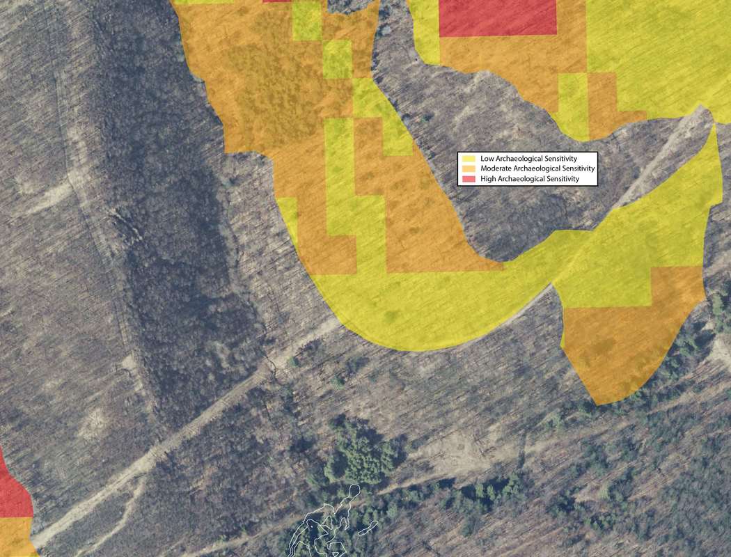 The methods for determining archaeological sensitivity vary by environmental setting but always take into consideration distance to water, soil type, slope and proximity to known archaeological resources. Areas within 100 meters of natural water courses are usually designated as high sensitivity and areas 300 meters are considered to be moderate, however; areas within those zones can be deemed low sensitivity if the percent of slope is greater than 15, or if the soil type is poorly drained. The details in GIS can be reserved for another discussion. Normally, archaeologists from each particular National Forest will develop their own sensitivity model for their forest as they know its environmental setting and existing conditions best. If one has not been developed, a statewide or regional model can be adopted if available or the contracting company will be required to develop their own model localized to the project area. Logging is common practice within National Forests. It is way to provide natural resources for the surrounding communities and the region. It is also a way to manage the forest by clearing areas with potential forest fire hazards and a way to promote new growth within the forest once the clearing is done. Logging, however, is disruptive to the soil as large machinery treads through the landscape and entire root structures are uprooted causing detrimental impacts to potential archaeological resources within the forest. A year prior to every scheduled round of clearing, the areas of impact are archaeologically surveyed. These areas of the forest are divided into small regions for clearing called Stands. Stand boundaries are mostly drawn on the basis of land forms, roadways or any other natural divide and can vary in size from about 10 to 60 acres. When an contracted archaeology firm takes on a project like this, they are provided a polygon shapefile of scheduled Stands numbering from about 80 to 100 at varying acreage and a polygon shapefile of the three tiered sensitivity zones covering the project area. GIS specialists for the company are then tasked with applying the sensitivity model to the Stands and generating shapefile point data representing shovel test pit locations respective to each zone of sensitivity within each Stand. These points number into the thousands. Each location is to be assigned a 5 digit Stand indentification number coupled with its unique accession number within each stand. The points are then converted into a waypoint file to be loaded into a Trimble Geo7X series GPS unit for sub-meter accuracy as per Forest Service requirements. In my experience as a GIS specialist for a CRM firm, having adopted this task two years ago, the process for generating these data points involved individual geoprocesses taking many arduous man hours that will be explained through the construction of a tool in ArcGIS Model Builder that now takes mere few seconds to execute. The tool accepts only two parameters, the two polygon shapefiles that are provided by the National Forest Service: Scheduled Stands and the Sensitivity Model. By inputting the two shapefiles, the tool begins by creating an arbitrary 100 meter buffer around the Stands parameter for the purposes of being able to manually shift the vertices of the lattice grid generated from the fishnet tool after the tool is run to overlay the centroid points also generated from the tool prior to clipping the lattice to the stand boundaries. The buffer is than used as a spatial template for the extent of two separate fishnets, one generating a 15 meter interval grid and the other generating a 30 meter interval grid. The fishnet tool generates a polygon or polyline grid at a specified interval and when checked will also generate centroid point for each box of the grid that can be the basis for shovel test pit locations. The 30 meter grid lattice is sent to the scratch folder as it will not be needed. The resulting 15 and 30 meter grid points are then sent to separate clipping functions. These clipping functions can not operate until parallel resulting preconditions are met. The preconditions are set by the sensitivity model parameter which first must be converted to a feature layer using the Make Feature Layer tool so that the Select tool maybe used twice upon its output. One selection would include high sensitivity attributes and the other would include only moderate sensitivity attributes. Then the two separate Clipping processes may begin with the "Use only selected features" box checked. The 15 meter interval Fishnet points will be clipped to the selected high sensitivity feature and the 30 meter points clipped to the selected moderate sensitivity feature. 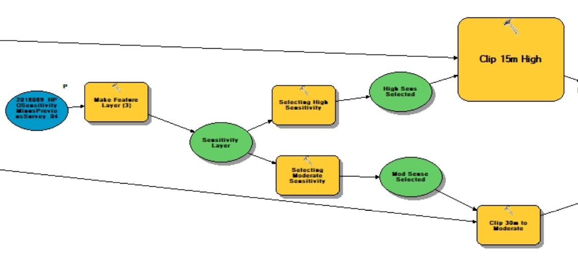 The results of each clipping process are then merged together using the Merge tool into one feature layer that consists of 15 meter interval points coinciding with high sensitivity zones and 30 meter interval points coinciding with moderate sensitivity zones. This output contains the number of points that will represent the number of shovel test pits required to fulfill the permit for clearing the scheduled Stands. The next process in the function is the Add Field tool. This will add an attribute field to the current feature that will represent each point's unique identifier within the Stand. The added field is an integer numeric data type that the result of which will again, be made into a new feature layer using the Make Feature Layer tool so hat it may be selected upon based on an iteration of the the individual Stands within the Stands layer. Here, the current layer is stopped until another precondition is met from a parallel running process that also involves the input parameter of the Stands shapefile. This part of the parameter is fed into a Select by Row iterator provided as a built-in function of Model Builder. This will iterate, like a for loop, through each record (Stand) after being converted into a feature layer. Every iteration will be input into the Select Layer by Location tool which will then select the inputted paused for preconditioned STP points layer as the taget and the selected Stand layer as the source. Each selected set of points will then be sent to the Calculate Field tool which, through a python expression, will add from low north to high east consecutive numbers the points layer per Stand. The expression is as follows: rec=0 def autoInc(): global rec if rec==0: rec=1 else: rec+=1 return rec Now every point within each Stand is assigned its own identifier in the drawing order that is easy to interpret in a field map. To assign the the Stand identifier to each point the Stand parameter through the iteration tool is then fed into the Spatial Join tool that takes the STP points layer as the target and the Stand as the join feature. Now every point has its respective 5-digit Stand code obtained by the attribute table from the Stand layer. Next, using the Delete Field tool, all fields existing in the resulting layer are deleted except for the the auto-incremented numbers field and the Stand identifier field. The Add Field tool is than used to make a string field of 10 characters called "test". The result of that is then fed into the Calculate Field where a simple concatenation python function <!STAND_ID! + "-"+str(!num!)> populates the field with every point's unique identifier-"#####-#". Now, by opening a single tool and inputting just two parameters,, a task that, in the past, took several hours now takes just under 45 seconds. 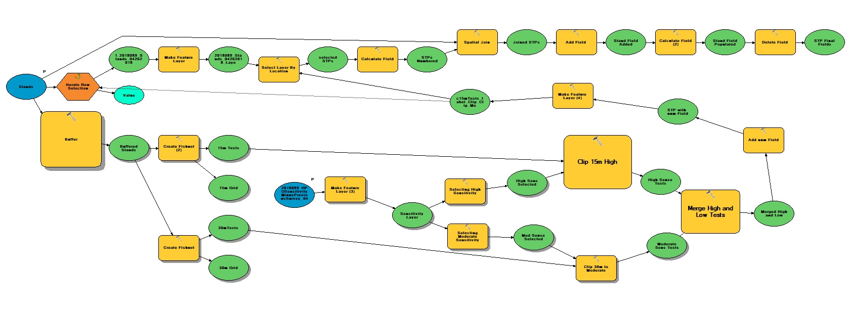
0 Comments
One of the most common ways to begin an archaeological investigation in the Eastern United States is in the form of a Phase IB survey. After an initial assessment of the project area, a IB may take the form of a pedestrian survey in which archaeologists comb the landscape in an evenly spaced formation looking to identify site indicative artifacts on the surface of the ground. This method usually only occurs if environmental settings consisted of tilled earth or a barren landscape. The other method would be to perform a series of evenly spaced shovel test pits in a grid fashion blanketing the project area or areas of assumed high to moderated archaeological sensitivity. The purpose of a shovel test pit (STP) is to sample a project area at evenly spaced intervals or at judgemental locations. An (STP), on average, is likely to be an approximately 1.5' diameter hole excavated in the ground to about one meter or 3.5' before impasse. Levels of provenience can either be determined by the natural stratigraphy or by any arbitrary increment. An STP in shape, can be round to square, but in any way it is best represented as point geometry type in terms locational sampling and mapping. The spacing of a test pattern grid is usually 50 feet or 15 meters and as seen in the example below. 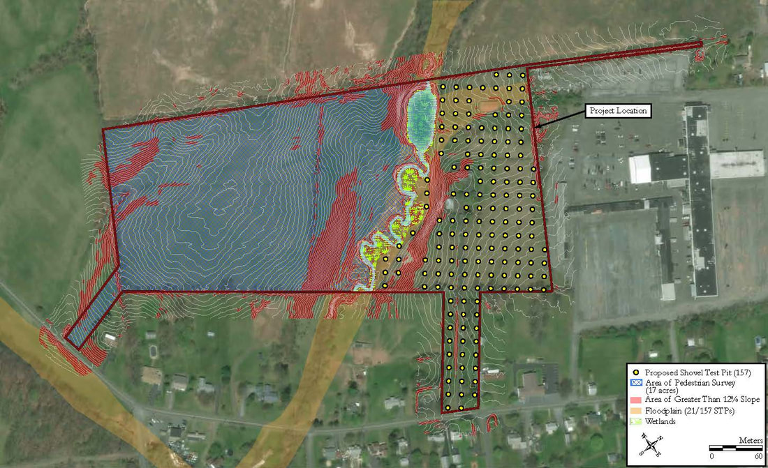 In the Olden Days, prior to survey, plots like these would be produced by hand with ruler and pencil on a set of scaled project plans and used in the field as a basis for the locations of shovel tests. With the advance of GIS software it became easier to produce a testing grid on a map by georeferencing project plans and using software tools, such as in ArcGIS, the Fishnet tool to produce a grid formation over a project area. The Fishnet tool was originally designed to create rectangular sampling polygons or polyline divisions at specified dimensions over a specified location. The output also includes center point data for every sampling polygon produced. The point feature can then be spatially moved, in an editing session, to meet the vertices of the intersecting lines or polygons to make a grid testing pattern precisely like ones used in a Phase IB survey. The points generated from this process come with zero attributes and no field to label each test. There are generally two ways to label or assign names to shovel test pits. One way is alphanumerically, in which STPs are assigned number, letters or a combination of the two across the testing grid. The other naming convention is to assign an arbitrary system of local grid coordinates to the testing pattern usually by northing and easting and always at the unit of measure and intervals on which the testing pattern was created such as N50/E50 and so on. 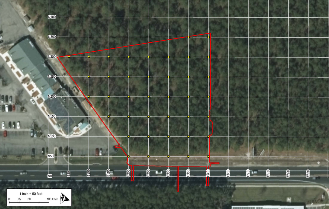 The latter is the preferred way for archaeologists conducting the survey in the field for a few reasons. The first is that by labeling only the grid lines there is no need to clutter up the map with labels for every test. Larger projects than the example above are displayed at larger scales thus shortening the perceived interval of the grid leaving little room for labels or notations on the map. Another reason that is that every STP name is also a locational descriptor of where the test is in the project area which is useful when referring to find spots. It is also helpful in keeping track of STPs prior to and before excavation, especially if you find yourself without a map. When a grid is labeled numerically, the direction of the testing transect may not always line up with the direction of the number increments and from test to test would be cutting across large and sometimes unpatterned number intervals.
The coordinate naming system, however; was not the preferred way for GIS and graphics specialists at the CRM firm I work for. It is easy to generate incremented numbers for every point in the testing grid using the snippet of python code, but a little more tricky to label every line in the grid and even more tedious to label every point in a shapefile with a name like "N2050/E1400" especially on larger projects that may have as many as 100 transects in either direction. If not entered manually test by test, shapefiles for these kinds of shovel tests usually were left unlabeled in their attributes and therefor the results of the STP were left out of the attribute table as well. For report graphics every grid line was labeled in post production, as task sometimes taking several hours to complete. Upon joining the GIS team, it was my goal to figure out a way to solve this problem. I had to develop a new way of thinking about this generated point data. Instead of having the fishnet tool create a series of evenly spaced points without attributes for you, why not plot the points yourself using grid coordinates as XY data. In Microsoft Excel, I made a a CSV of three fields. The first field was for the Northing value, the second for Easting and the third for a concatenation of the two values that include a letter "N" at the beginning and a "/E" dividing them. The table had to be big, big enough to accommodate project areas that could be 10,000 feet in either direction. Using the powers of the software I was able to quickly produce a table of point values starting at 0,0 for over 40,000 points and the concatenation of the point values for name assignment. This was done at increments of 50 for projects that require intervals in feet and one with increments of 15 for projects that require intervals in meters. In ArcMap I plotted the tables as CSV events in a state plane coordinate reference system for New Jersey in feet and Pennsylvania North and South in meters. The points plotted beginning at the 0,0 point of the projected CRS and the events were exported as shapefiles to their respective coordinate reference systems. For grid lines I still needed to rely on the fishnet tool but by selecting vertical lines apart from horizontal lines and using the python defined auto increment function in the field calculator was able to increment them according to their interval spacing instead of by 1. A string concatenation in an added field called "Transect" allowed me to include and "N" for horizontal lines and an "E" for vertical lines. The resulting grid was moved to be placed with the line vertices matching precisely with their corresponding points plotted from the CSV. Now there is a template on the company server that consists of shapefiles of grid lines and points for the three most common projected CRSs. They can be brought into any GIS project and be positioned and oriented over a project area with the label assignment for points and lines already complete. Results from the shovel tests can now also be quickly joined from a Shovel Test Pit Log, in all saving the company several hours per project. |
 RSS Feed
